Let's go and explore some publicly available climate data about germany and draw some meaningful conclusions from that.
the data source
The german weather service, called DWD, publishes a vast amount of data measured at german weather stations. The data is available in monthly, daily and hourly intervals, partly from the beginning of recorded official measurements. Temperature, humility, cloudiness, precipitation, air pressure, soil temperature, sunshine duration, radiation, wind speed and direction and sun zenith are measured. Not all stations provide measurements for all those categories.
I created some python scripts to download and convert the DWD data from their FTP server into json files suited for import into the CRATE database. The source code and detailed instructions on how to download and convert the data yourself is available on my Github Repository.
I converted the source dataset from the DWD so that all measurements at a station and a point in time make up one row. It now consists of around 236 mio. rows.
the database
Well, I chose CRATE to showcase this dataset partly because i helped building it and want to show how awesome both the dataset and the database are. Partly it was necessary to have a fast and performing database with capabilities to analyze the dataset without doing it all on client side.
Well, CRATE is just fine for that purpose. It is a distributed database, making use of replication and sharding, so we can make good use of all nodes in the database cluster and expect good scalability. It is open source and available at Github . CRATE supports all common SQL features applicable on a single relation / table besides subselects (as of this writing). This includes GROUP BY queries using aggregations on a distributed dataset. Even an exact COUNT(DISTINCT ...) is possible (given enough servers).
the data
To get our hands dirty on the dataset, we use crash , the CRAte SHell.
We have around 236 mio. rows in total from 1455 different stations:
cr> SELECT COUNT(*), COUNT(DISTINCT station_id)
... FROM german_climate_denormalized;
+-----------+----------------------------+
|  count(*) | count(DISTINCT station_id) |
+-----------+----------------------------+
| 235603810 |                       1455 |
+-----------+----------------------------+
SELECT 1 row in set (66.984 sec)
The earliest measurements were taken way back at the beginning of 1891 by stations in Kiel, Marburg and Kassel:
cr> SELECT date_format('%Y-%m-%d', min(date)) AS min_date, station_name
... FROM german_climate_denormalized
... GROUP BY station_name
... ORDER BY 1, 2 ASC
... LIMIT 10;
+------------+---------------------+
| min_date   | station_name        |
+------------+---------------------+
| 1891-01-01 | Kassel-Harleshausen |
| 1891-01-01 | Kiel-Kronshagen     |
| 1891-01-01 | Marburg-Cappel      |
| 1893-01-01 | Potsdam             |
| 1901-01-01 | Königstuhl          |
| 1921-01-01 | Witzenhausen        |
| 1926-01-01 | Bremen              |
| 1936-01-01 | Wrixum/Föhr         |
| 1937-01-01 | Aachen              |
| 1937-01-01 | Braunlage           |
+------------+---------------------+
SELECT 10 rows in set (63.527 sec)
The station joining in at last was Freiberg in 2015-04-01 and the last measurement was taken at 2015-05-17 23:00:00 (UTC) at several stations which is about the time I downloaded and converted the dataset (around end of may 2015).
If you download and convert the data yourself, there might be more and newer data available, as the DWD seems to regularly update their stuff (Last update seems to have been 2015-07-01 as of this writing).
too slow
Have you seen how long it took, to get those earliest measurements?
More than 60 seconds!!!
That is not acceptable. Clearly not! 60 seconds for aggregating a little more than 240 million records. Pah!
I've deployed the dataset on a CRATE cluster of 3 nodes hosted on amazon EC2. These are m3.xlarge instances with 4 cores @ 2.5 GHz and 14 GB of RAM. The data folder resides on an EBS SSD.
The CRATE admin UI reports that we only use around 1-2 GB out of available 10 GB of configured heap. So we seem to be CPU and/or disk bound. So let's add more of those.
I've added another node with the exact same configuration, so we have 4 nodes now:
cr> select count(*) from sys.nodes;
+----------+
| count(*) |
+----------+
|        4 |
+----------+
SELECT 1 row in set (0.001 sec)
After some waiting time, we can see that all nodes got a nearly equal number of shards:
cr> select _node['name'], id, "primary", num_docs from sys.shards where primary=true and table_name='german_climate_denormalized';
+---------------+----+---------+----------+
| _node['name'] | id | primary | num_docs |
+---------------+----+---------+----------+
| ElectroCute   |  3 | TRUE    | 20356276 |
| ElectroCute   |  6 | TRUE    | 24011877 |
| ElectroCute   |  9 | TRUE    | 18035793 |
| Coldblood     | 11 | TRUE    | 20594732 |
| Coldblood     |  5 | TRUE    | 21583310 |
| Coldblood     |  8 | TRUE    | 24234462 |
| Stem Cell     |  2 | TRUE    | 22271198 |
| Stem Cell     |  0 | TRUE    | 19469386 |
| Arclight      | 10 | TRUE    | 18361742 |
| Arclight      |  1 | TRUE    | 16693415 |
| Arclight      |  7 | TRUE    | 14902349 |
| Arclight      |  4 | TRUE    | 15089270 |
+---------------+----+---------+----------+
SELECT 12 rows in set (0.004 sec)
The query for the earliest measurements now runs quite a bit faster:
cr> SELECT date_format('%Y-%m-%d', min(date)) AS min_date, station_name
... FROM german_climate_denormalized
... GROUP BY station_name
... ORDER BY 1, 2 ASC
... LIMIT 10;
+------------+---------------------+
| min_date   | station_name        |
+------------+---------------------+
| 1891-01-01 | Kassel-Harleshausen |
| 1891-01-01 | Kiel-Kronshagen     |
| 1891-01-01 | Marburg-Cappel      |
| 1893-01-01 | Potsdam             |
| 1901-01-01 | Königstuhl          |
| 1921-01-01 | Witzenhausen        |
| 1926-01-01 | Bremen              |
| 1936-01-01 | Wrixum/Föhr         |
| 1937-01-01 | Aachen              |
| 1937-01-01 | Braunlage           |
+------------+---------------------+
SELECT 10 rows in set (39.534 sec)
Several attempts show constant results all taking around 40 seconds. We got a speedup of one third of the initial time.
Well that is much nicer!
Like this I'll get this blog post done much faster.
some random results
The day with the hottest temperature ever measured:
cr> SELECT date_format('%Y-%m-%d', DATE_TRUNC('day', date)) AS day, MAX(temp) as max
... FROM german_climate_denormalized
... WHERE temp IS NOT NULL
... GROUP BY 1
... ORDER BY 2 DESC
... LIMIT 1;
+------------+------+
| day        |  max |
+------------+------+
| 1993-03-25 | 49.1 |
+------------+------+
SELECT 1 row in set (55.948 sec)
According to the following query the wind of change blew peacefully with a speed of around 10 m/sec with direction SW the evening of the fall of the berlin wall near the brandenburg gate:
cr> SELECT station_name, position, date_format('%Y-%m-%d %T', date) as date, wind_direction, wind_speed
... FROM german_climate_denormalized
... WHERE date > '1989-11-09T18:00:00+02:00' AND date < '1989-11-10T06:00:00+02:00'
... AND DISTANCE('POINT(52.51628 13.37754)', position) < 30000
... ORDER BY german_climate_denormalized.date ASC;
+--------------------------+--------------------+---------------------+----------------+------------+
| station_name             | position           | date                | wind_direction | wind_speed |
+--------------------------+--------------------+---------------------+----------------+------------+
| Berlin-Buch              | [52.6325, 13.5039] | 1989-11-09 17:00:00 |           NULL |     NULL   |
| Berlin-Tegel             | [52.5642, 13.3086] | 1989-11-09 17:00:00 |            230 |        4.6 |
| Berlin-Schönefeld        | [52.3822, 13.5325] | 1989-11-09 17:00:00 |            250 |        6.0 |
| Berlin-Tempelhof         | [52.4672, 13.4019] | 1989-11-09 17:00:00 |            250 |        4.7 |
| Berlin-Alexanderplatz    | [52.5206, 13.4106] | 1989-11-09 17:00:00 |            250 |       10.0 |
| Berlin-Dahlem (FU)       | [52.4639, 13.3017] | 1989-11-09 17:00:00 |           NULL |     NULL   |
| Berlin-Alexanderplatz    | [52.5206, 13.4106] | 1989-11-09 18:00:00 |            270 |       11.0 |
| Berlin-Tegel             | [52.5642, 13.3086] | 1989-11-09 18:00:00 |            240 |        2.6 |
| Berlin-Buch              | [52.6325, 13.5039] | 1989-11-09 18:00:00 |           NULL |     NULL   |
| Berlin-Tempelhof         | [52.4672, 13.4019] | 1989-11-09 18:00:00 |            240 |        2.8 |
| Berlin-Schönefeld        | [52.3822, 13.5325] | 1989-11-09 18:00:00 |            230 |        3.0 |
| Berlin-Dahlem (FU)       | [52.4639, 13.3017] | 1989-11-09 18:00:00 |           NULL |     NULL   |
| Berlin-Schönefeld        | [52.3822, 13.5325] | 1989-11-09 19:00:00 |            210 |        3.0 |
| Berlin-Dahlem (FU)       | [52.4639, 13.3017] | 1989-11-09 19:00:00 |           NULL |     NULL   |
| Berlin-Alexanderplatz    | [52.5206, 13.4106] | 1989-11-09 19:00:00 |            280 |       12.0 |
...
| Berlin-Schönefeld        | [52.3822, 13.5325] | 1989-11-10 03:00:00 |            180 |        2.0 |
| Berlin-Dahlem (FU)       | [52.4639, 13.3017] | 1989-11-10 03:00:00 |           NULL |     NULL   |
| Berlin-Buch              | [52.6325, 13.5039] | 1989-11-10 03:00:00 |           NULL |     NULL   |
| Berlin-Tempelhof         | [52.4672, 13.4019] | 1989-11-10 03:00:00 |            210 |        1.0 |
| Berlin-Alexanderplatz    | [52.5206, 13.4106] | 1989-11-10 03:00:00 |            250 |        5.0 |
| Berlin-Tegel             | [52.5642, 13.3086] | 1989-11-10 03:00:00 |            180 |        1.3 |
+--------------------------+--------------------+---------------------+----------------+------------+
SELECT 57 rows in set (0.439 sec)
No wonder it all happened as it finally did!
I think this weather thing is a way better kind of horoscope, though it only works in retrospective.
about climate change
Let's do some serious stuff!
It's definitely getting hotter:
The 20 warmest years in the historical record have all occurred in the past 20 years. Except for 1998, the 10 warmest years on record have occurred since 2002.
This site also states that 2014 was the hottest year (globally) since records began in 1880.
Is that also true for Germany? Or do we get different results here? Might it even get colder?
Let's see. At first let's get the 20 warmest years for whole germany by taking the average of all measurements:
cr> SELECT AVG(temp) AS avg_temp, date_format('%Y', date) AS year FROM german_climate_denormalized
... WHERE temp IS NOT NULL
... GROUP BY 2
... ORDER BY 1 DESC
... LIMIT 20;
+--------------------+------+
|           avg_temp | year |
+--------------------+------+
| 10.383287611870998 | 1934 |
| 10.294091249625682 | 2014 |
|  9.77962916625624  | 2007 |
|  9.608534610942437 | 2011 |
|  9.54839722179719  | 2006 |
|  9.517990867210951 | 1911 |
|  9.473769719418058 | 2000 |
|  9.448253424433336 | 1921 |
|  9.425364196579832 | 2008 |
|  9.366613391466167 | 1943 |
|  9.356940640983721 | 1938 |
|  9.34618359753395  | 1994 |
|  9.288165251974975 | 2002 |
|  9.242351867189395 | 2003 |
|  9.20187707133279  | 1989 |
|  9.193755711258717 | 1926 |
|  9.17595889954296  | 1945 |
|  9.147633379946301 | 2009 |
|  9.123652967148924 | 1930 |
|  9.115169487073727 | 1990 |
+--------------------+------+
SELECT 20 rows in set (41.357 sec)
Well only 9 out of 20 of the warmest years seem to be among the last 20.
But wait, that was too easy. Do we have enough measurements for all those years? If some period is missing, we might get a wrong result. Do we have the same amount of data for every year for every station? If we have more data from the alps, than from the baltic sea we might also get strange results.
So lets explore our data a little bit more.
At first, every year has got some temperature data missing:
cr> SELECT date_format('%Y', date) AS year FROM german_climate_denormalized
... WHERE temp IS NULL
... GROUP BY 1
... ORDER BY 1 DESC;
+------+
| year |
+------+
| 2015 |
| 2014 |
| 2013 |
| 2012 |
| ...  |
| 1891 |
+------+
SELECT 125 rows in set (43.247 sec)
Well fuck! Is there at least one station with temperature data for every year? Or at least with "enough" data to be meaningful? For example for the whole 20th century?
The following query shows us that we indeed have some stations with sufficient data. To keep it simple and this blog post short, lets only check for the data of the station in Potsdam. Here we have enough data spread across the whole century and its quite near where I live:
cr> SELECT COUNT(*) - COUNT(temp) AS missings, COUNT(*) AS "all", date_format('%Y', MAX(date)) AS min, date_format('%Y', MAX(date)) AS max, station_name
... FROM german_climate_denormalized
... GROUP BY station_name
... ORDER BY 1 ASC;
+----------+---------+------+------+-----------------------------------------+
| missings |     all |  min |  max | station_name                            |
+----------+---------+------+------+-----------------------------------------+
|        0 |   70128 | 1947 | 1955 | Bamberg (Sternwarte)                    |
|        0 |   89517 | 2005 | 2015 | Falkenberg,Kr.Rottal-Inn                |
...
|       14 | 1072704 | 1893 | 2015 | Potsdam                                 |
...
|   660817 |  660817 | 1891 | 2005 | Marburg-Cappel                          |
+----------+---------+------+------+-----------------------------------------+
SELECT 1455 rows in set (59.519 sec)
So let's check potsdam:
cr> SELECT AVG(temp) AS avg_temp, date_format('%Y', date) AS year FROM german_climate_denormalized
... WHERE temp IS NOT NULL AND station_name = 'Potsdam'
... GROUP BY 2
... ORDER BY 1 DESC
... LIMIT 20;
+--------------------+------+
|           avg_temp | year |
+--------------------+------+
| 10.976700911312003 | 2014 |
| 10.524235156003266 | 2007 |
| 10.404178055522383 | 2000 |
| 10.383287611870998 | 1934 |
| 10.26071265868025  | 2008 |
| 10.192248860258422 | 2011 |
| 10.180684938320049 | 1999 |
| 10.168687218542479 | 2006 |
| 10.07344749342208  | 1989 |
| 10.021700914364018 | 1990 |
|  9.843116434962068 | 1994 |
|  9.835308221788848 | 1983 |
|  9.81356028513564  | 1992 |
|  9.803527404431714 | 1953 |
|  9.770022827612244 | 2003 |
|  9.74616438152192  | 1949 |
|  9.744703196483286 | 2002 |
|  9.7272085620545   | 1948 |
|  9.645662097751108 | 2009 |
|  9.640216891846904 | 1975 |
+--------------------+------+
SELECT 20 rows in set (0.983 sec)
We do have 10 out of 20 years within the last 20 years, now with a proper amount of backing data. For Potsdam, local average temperature during the last 20 years is below the global average. But 2014 has been the warmest year since records began for Potsdam as well.
Let's end this post with something at least a little bit more beautiful, at least visually. I'd like to compare the potsdam data against the graph on climate.gov showing the deviation from the global mean from the 20th century.
Let's first get the mean for potsdam:
cr> SELECT AVG(temp) AS avg_temp
... FROM german_climate_denormalized
... WHERE temp IS NOT NULL AND station_name = 'Potsdam'
... AND date > '1900-01-01' AND date < '2000-01-01';
+-------------------+
|          avg_temp |
+-------------------+
| 8.659611756762368 |
+-------------------+
SELECT 1 row in set (0.860 sec)
In the next step, we get the deviation:
cr> SELECT date_format('%Y', date) AS "year", AVG(temp) - 8.659611756762368 as "deviation"
... FROM german_climate_denormalized
... WHERE temp IS NOT NULL AND station_name = 'Potsdam'
...       AND date < '2015-01-01' -- exclude 2015, as there is not enough data yet
... GROUP BY 1
... ORDER BY 1 ASC;
+------+-----------------------+
| year |             deviation |
+------+-----------------------+
| 1893 | -0.6210114614387638   |
| 1894 | -0.2302966852799706   |
| 1895 | -0.785970202273317    |
| 1896 | -0.588971957632193    |
| 1897 | -0.5678195145597495   |
| 1898 |  0.18216906134509792  |
| 1899 | -0.21009121009924137  |
| 1900 | -0.016803531999752153 |
| 1901 | -0.583047827430569    |
| 1902 | -1.6493035382361265   |
...
| 2009 |  0.98605034098874     |
| 2010 | -0.32656380951223163  |
| 2011 |  1.5326371034960538   |
| 2012 |  0.9353677540863323   |
| 2013 |  0.7654681501021567   |
| 2014 |  2.3170891545496346   |
+------+-----------------------+
SELECT 122 rows in set (1.156 sec)
And for the last step we now need some R magic to turn this data into some beautiful bar graph:
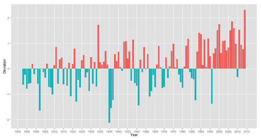
As we can see, it follows the same tendency as the global graph.
final words
Well at first I hope, you finally made it here, and if so, congrats for you epic patience! Secondly, I hope some of my pleasure regarding real life datasets like this one about the german weather somehow swapped over to you. And finally maybe you realized how awesome CRATE really is.
To be continued...
appendix
importing the data
Here are the SQL statements that can be used to import the weather data to your own CRATE cluster.
At first the table schema needs to be created with the following statement, also available as SQL CREATE TABLE script:
CREATE TABLE german_climate_denormalized (
  date timestamp,
  station_id string,
  station_name string,
  position geo_point, -- position of the weather station
  station_height int, -- height of the weather station
  temp float, -- temperature in °C
  humility double, -- relative humulity in percent
  cloudiness int,  -- 0 (cloudless)
                   -- 1 or less (nearly cloudless)
                   -- 2 (less cloudy)
                   -- 3
                   -- 4 (cloudy)
                   -- 5
                   -- 6 (more cloudy)
                   -- 7 or more (nearly overcast)
                   -- 8 (overcast)
                   -- -1 not availavle
  rainfall_fallen boolean, -- if some precipitation happened this hour
  rainfall_height double,  -- precipitation height in mm
  rainfall_form int, -- 0 - no precipiation
                     -- 1 - only "distinct" (german: "abgesetzte") precipitation
                     -- 2 - only liquid "distinct" precipitation
                     -- 3 - only solid "distinct" precipitation
                     -- 6 - liquid
                     -- 7 - solid
                     -- 8 - solid and liquid
                     -- 9 - no measurement
  air_pressure double,  -- air pressure (Pa)
  air_pressure_station_height double, -- air pressure at station height (Pa)
  ground_temp array(float), -- soil temperature in °C at 2cm, 5cm, 10cm, 20cm and 50cm depth
  sunshine_duration double, -- sum of sunshine duration in that hour in minutes
  diffuse_sky_radiation double, -- sum of diffuse short-wave sky-radiation in J/cm² for that hour
  global_radiation double, -- sum of global short-wave radiation in J/cm² for that hour
  sun_zenith float, -- sun zenith in degree
  wind_speed double, -- wind speed in m/sec
  wind_direction int -- wind direction given in degrees (90=E, 180=S, ...)
) clustered by (station_id) into 12 shards with (number_of_replicas=0, refresh_interval=0);
If you want to download and recreate the dataset yourself, use my Github Repository. All steps are explained in detail there.
In order to get the data into your CRATE cluster you need to issue a COPY FROM command. You can COPY FROM a local (to the database cluster) dataset on filesystem or from S3.
For further information on the exact syntax and usage of COPY FROM take a look at the Crate documentation about importing huge datasets and the COPY FROM reference .
As last step, when COPY FROM finally finished its import job, you need to refresh the table to make all the data available for all kinds of queries:
REFRESH TABLE german_climate_denormalized;
Now you can finally reproduce what i did above and much more. Have fun!
public dataset
I made the dataset (downloaded and converted around the end of may 2015) publicly available in an amazon s3 bucket. CRATE supports importing and exporting data from and to s3. Here you go:
COPY german_climate_denormalized FROM 's3://crate.sampledata/climate_germany/denormalized/*.json.gz' with (compression='gzip');